Computer Vision: Object Detection

This is the third post in our computer vision blog series. In the first entry we focused on what computer vision is and how the computer sees an image, and in the second entry on what convolutional neural networks are and how they work. Now it’s time to dive into object detection, which is probably the most common application of computer vision nowadays.

What is object detection?

Although object detection was shortly covered in the first post of this series, it’s always good to recap. The goal of object detection, as the name suggests, is to locate and classify instances of objects in images or videos. Classification refers to the assignment of a category label from a known set of categories, and localisation refers to predicting the location of an object instance within the image or video frame (which is basically just an image). Modern object detection methods are based on deep learning, which is what we’ll focus on in this post. We’ll go through the main concepts of modern deep learning based object detection methods, and then look at one of the most well known object detection algorithms, called YOLOv3 (You Only Look Once, version 3).

Bounding box prediction

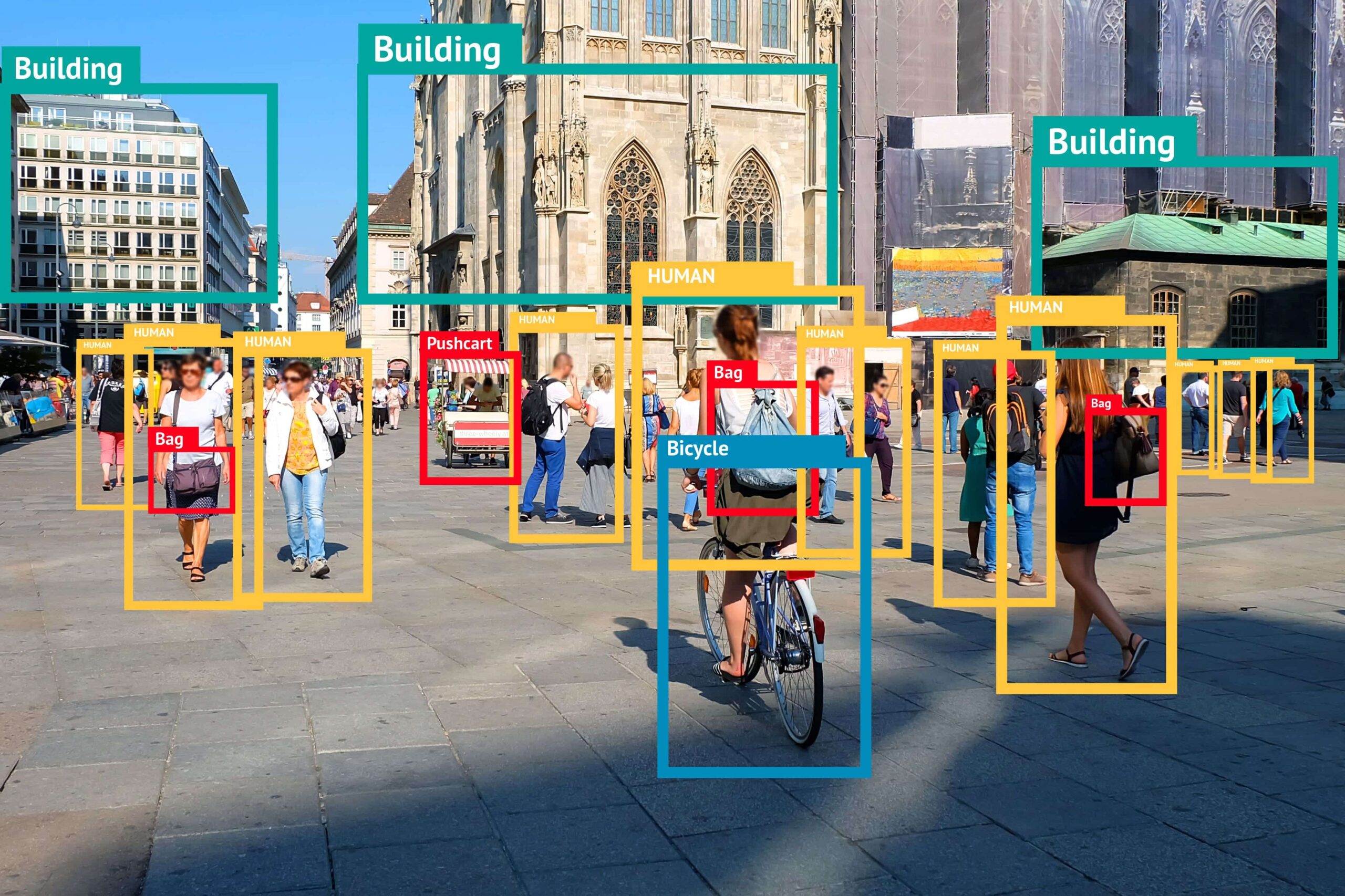
Locating objects in an image is a regression problem. Regression refers to the prediction of a real-valued quantity, which in this case is the relative coordinates of an object in a given image defined by a bounding box. A bounding box has four coordinates, the centre point of the object (x, y) and the width and height of the box (w, h). A bounding box is what you can see in Figure 1, the red and blue boxes.

A bounding box prediction is basically, and for the sake of simplicity, generated by convolving over the image, as discussed in the previous post, and classifying each convolved region either as object or no object. This, however, means that the total number of potential bounding boxes per image is much larger than the number of actual bounding boxes because object detectors usually output many overlapping bounding boxes for the same object. Each bounding box prediction, however, has an associated confidence score that indicates how certain the model is that there is an object within that particular bounding box (remember, object or no object).

Intersection over union

So, how do we know if a predicted bounding box is good or not? The good thing is that we know the groundtruth (a target assigned by a human), that is, we know where the correct bounding box is located for that particular object. To improve bounding box predictions, we need to apply an algorithm called intersection over union (also known as the Jaccard index). 

Intersection over union (IoU) is defined as the area of intersection divided by the area of union of the groundtruth and the predicted bounding box. The closer the IoU score is to 0, the worse the predicted bounding box is, and the closer the score is to 1, the better the predicted bounding box is. Pretty straightforward in the end. IoU is used in the loss function at training time to refine bounding box predictions.

Non-max suppression

As mentioned above, object detectors often output several overlapping bounding boxes for each object. Lucky for us, each bounding box has an associated confidence score. So, to filter out the suboptimal boxes, we need to apply a post-processing algorithm called non-max suppression (NMS). Like with IoU (that is, intersection over union as described above), the name of the algorithm already basically says what it’s all about.

The non-max suppression algorithm starts by selecting the bounding box with the highest confidence score (the closer to 1, the better). It uses that bounding box as the final prediction. Then it computes the IoU of the remaining boxes with respect to the box it selected, so the one with the highest confidence score. It then discards all boxes that have a higher IoU than some specified threshold (0.5 or higher, usually).

Now, one might ask why do we go through all this trouble instead of just picking the bounding box with the highest confidence score and discarding the rest, why compute the IoU in the first place? Well, we don’t know how many objects there are present in a given image, and NMS addresses that issue by removing redundant bounding box predictions, and this is also why we need to define an IoU threshold. If the IoU score is smaller than the threshold, then that bounding box most likely belongs to another object present in the same image.

Anchor boxes

Anchor boxes are dimension priors, meaning that they are bounding boxes that encode the most common and descriptive N dimensions (N is an integer number that depends on the object detector) of the objects in the training dataset. Before anchor boxes were hand-picked, but since YOLO9000 (aka YOLOv2, by the authors of YOLOv3), they are generated from the training dataset using K-means clustering (how it works exactly is out of the scope of this blog post but there are plenty of good articles about it on the internet).

The main advantage of anchor boxes is that detecting overlapping objects of different dimensions is much easier. Before training, each object in the training dataset is assigned a corresponding anchor box with the highest IoU. This improves the prediction accuracy because the detector basically learns which dimensions are associated with different types of objects. For example, it learns that cars are generally of a certain shape and size and humans are of different shape and size. So, basically, the more anchor boxes a detector uses, the better predictions it can make. However, if two objects of the same shape and size overlap, well, too bad.

YOLOv3

Now that we know the main concepts of object detection, let’s look at YOLOv3 and see how they all come together. Let’s start with the bounding box prediction. YOLOv3 predicts boxes at three different scales, so it downsamples the same image by factors of 32, 16, 8, meaning that if the image is of size 416×416, the downsampled feature maps, or grids (Figure 4 illustrates a 3×3 grid using the black lines going through the image horizontally and vertically), are 13×13, 26×26, and 52×52 respectively. Each scale has its associated anchor boxes. All this scaling stuff is done because not all objects are easily detected at the same scale. For example, smaller objects tend to have better anchors at a smaller scale. The centre point of an object is assigned to its corresponding grid cell (centre grid cell in Figure 4), as well as the associated anchor box and groundtruth.

Essentially, the grids are multidimensional matrices of zeros except for the dimensions in which the centre points, anchors and groundtruths are stored, so to say. The first two dimensions of said matrices are the grid width and height, which is basically how YOLOv3 

knows in which grid there should be the centre of an object. So, let’s say we have a 3×3 grid as per Figure 4 and we have 3 classes as per Figure 5 (dog, bicycle, truck). YOLOv3 would output a vector of size 3x3x3x8, where the first two dimensions are the grid width and height, third dimension is the number of anchors per scale, and the last dimension – 8 in this example – includes the confidence (aka objectness) score, the centre coordinates x and y, the bounding box width and height (w, h), and the three different classes (hence, the last dimension is always of size 5 + number of classes). That output vector is then decoded to get the actual predictions. That’s pretty much it in a nutshell, just some algorithmic maths stuff, not magic.

For the class prediction of an object in a given bounding box, YOLOv3 uses binary cross-entropy loss, which doesn’t enforce mutually exclusivity. In other words, an object can belong to more than one class. How the class prediction is done was covered in the first blog post basically because it can be seen as a special case of image classification, which it kind of is. So, object detection algorithms classify the bounding boxes, not images.

Conclusion

Now that we’ve covered the basic concepts of computer vision, deep learning, and object detection, as well as how YOLOv3, one of the most famous object detection algorithms works, we are pretty much ready to get to the point of this blog series, which is our research. We just had to cover some of the basics (so to say) first, so that anyone who’s interested but lacks the background can more or less follow along.

Sources

[1] https://learnopencv.com/classification-with-localization/

[2] https://web.eecs.umich.edu/~justincj/slides/eecs498/498_FA2019_lecture15.pdf

[3] https://www.researchgate.net/figure/Non-Maximal-Suppression_fig5_345061606

[4] https://www.dlology.com/blog/gentle-guide-on-how-yolo-object-localization-works-with-keras-part-2/

[5] https://pjreddie.com/darknet/yolo/